Overview
This project is a C++ version of the A* pathfinding algorithm described by Ian Millington in his book AI for Games Third Edition.
It was the first more structured project done in C++ and it was the one that got me confident in the language; the majority of the code regarding the pathfinding was written in pair-programming.
The algorithm
Pathfinding algorithms solve a common problem of every video game: which is the best path (if there is one) between two points, where best means the less expensive one.
However they do not take into consideration nor the why or the how.
To represent the “level” we use a graph which is made of nodes and connections.
More precisely we represent it with a directed non-negative weighted graph:
- directed: each connection is one-way only (ex. point A to B but NOT point B to A);
- non-negative weighted: the cost of a connection can represent how much time the agent spends using that connection or how far the two nodes connected are or also how difficult that path is.
Node representation:
  struct Node
  {
    struct Point
    {
      float X;
      float Y;

      Point(float x, float y);
      Point(int x, int y);
    };

    int ID;
    Point Position;
    Node(int id, Point position);
  };
Connection representation:
  struct Connection
  {
    int From;
    int To;
    float Cost;

    Connection(int from, int to, float cost);
  };
A*
This algorithm, given a graph and two points (a start node and an end node), returns an array of connections to follow to go from the start node to the end node.
This path, theoretically, should be the less expensive one but, since this implementation is thought to be used in game development, we stop the algorithm once we reach the end node thus settling for one with a low cost rather than the least expensive one.
Broadly speaking, the algorithm checks all the connections of the current node (starting from the start one) and for each “To” node (the node that connection points to) stores:
the cost of the path until that moment (cost-so-far);
the node that connection started from;
the “estimated-total-cost” which is the sum of the cost-so-far and an estimate of the cost to go from that node to the end node into a struct “Node Record”
  struct NodeRecord
  {
    Graph::Node Node;
    Graph::Connection Connection;
    NodeRecord* ParentNode;
    float CostSoFar;
    float EstimatedTotalCost;

    NodeRecord();

    NodeRecord
    (
      Graph::Node node, Graph::Connection connection,
      NodeRecord* parentNode, float costSoFar,
      float estimatedTotalCost
    );
  };
This estimate is done by a “heuristic”, a function that calculates a value of how close that node is to the goal; choosing the right heuristic is one of the keys to make the most out of the A* algorithm.
In this implementation we decided to use a simple Euclidean distance.
Each newfound node is put in an “open array” and when all the connections of a node are checked we put it in the “closed array”; the algorithm goes on by selecting the node in the open array with the lower estimated-total-cost and making it the current node until it reaches the end node
Since we base the algorithm on an estimate, it could be wrong and there may be nodes in the closed array with a not accurate cost-so-far value.
That is why another key point of this algorithm is the possibility to update nodes in the closed array if we reach them again with a different path that has a lower cost-so-far value then the one it currently has.
Version #1: Array of open and closed nodes
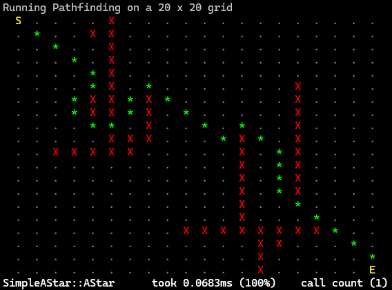
The first, simple, implementation of the algorithm stores all the information about the nodes inside two arrays, an open one and a closed one.
This approach was not the best one since the array as data structures were not the best choice: although inserting a new element has a time complexity of O(1), searching for the smallest node in the array and removing a specific node have a time complexity of O(n) which is not bad per se but potentially this arrays could contain hundreds of nodes, not the best.
Version #2: Node Array
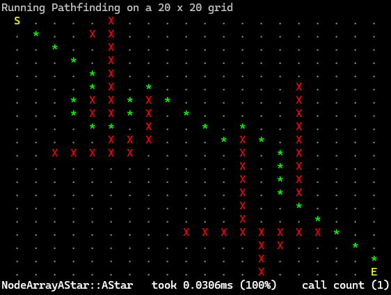
This is the implementation suggested by the author of the book and is generally faster and is based on a simple tradeoff: increasing the memory used at the beginning to improve execution speed.
We create for each node in the graph its node record structure which now looks like this:
  struct NodeRecord
  {
    enum State
    {
      OPEN,
      CLOSED,
      UNVISITED,
    };

    Graph::Node Node;
    Graph::Connection Connection;
    NodeRecord* ParentNode;
    float CostSoFar;
    float EstimatedTotalCost;
    State State;
    NodeRecord();

    NodeRecord(Graph::Node node, Graph::Connection connection, NodeRecord* parentNode, float costSoFar, float estimatedTotalCost);
  };
The “State” enum is used to get rid of the closed array since we can directly check the State in the Node Array created at the beginning, saving us the time to check the closed array.
Version #3: Heap Node Array of node records
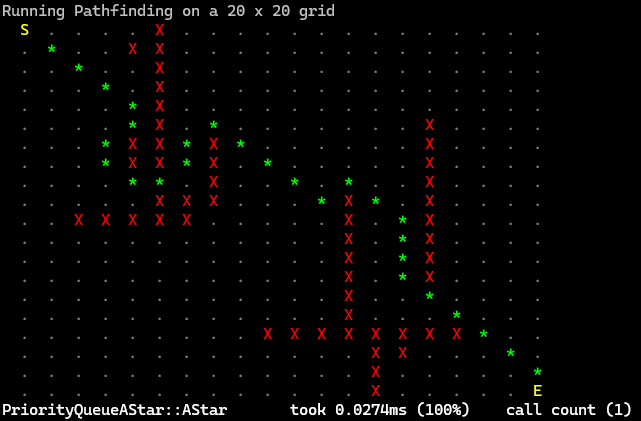
We still have a problem, we lose a lot of time in the process of finding the smallest element in the open list.
To overcome it, we substitute the data structure used to store the open nodes: from a simple array to a priority queue which has a worse time complexity adding and removing an item O(log n) but has a constant time complexity when retrieving the smallest node O(1).
This is because the data structure keeps all the elements in a given order and in our case the order is the “estimated-total-cost”.
auto cmp = [] (NodeRecord* left, NodeRecord* right)
{ return (left->EstimatedTotalCost) > (right->EstimatedTotalCost); };
std::priority_queue<NodeRecord*, std::vector<NodeRecord*>, decltype(cmp)> open(cmp);
Comparison
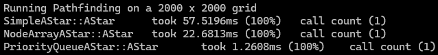
The comparison between the three versions is made with a 2000x2000 grid and shows significant improvements by using the priority queue with the NodeRecord structure suggested by the book.